Coding workshop: Week 6

1. Summary

Packages

• tidyverse
  
• lterdatasampler
  
• paletteer
  
• ggthemes
  
• tvthemes
  
• ggpomological
  
• gghighlight
  
• patchwork
  
• gganimate
  
• ggimage
  
• plotly

Operations

New functions

• use color palettes with paletteer::paletteer_c() and paletteer::paletteer_d()
  
• use themes from tvthemes (amongst other packages)
  
• highlight elements using gghighlight()
  
• make figures into gifs using gganimate::transition_reveal()
  
• insert images into figures using ggimage::geom_image()
  
• make figures interactive using plotly::ggplotly()

Review

Data sources

These are all datasets from the lterdatasampler package.

2. Code

1. Set up

library(tidyverse)
library(lterdatasampler)

# use color palettes
# if using paletteer:
library(paletteer)
# if not, insert color palette package here

# use theme packages to change plot aesthetics
# insert theme package here
library(ggthemes)
library(tvthemes)
library(ggpomological)

# highlight figure components
library(gghighlight)

# put multiple figures together
library(patchwork)

# make figures into gifs
library(gganimate)

# insert images into plots
library(ggimage)

# make figures interactive
library(plotly)

Run this to see datasets from lterdatasampler in your environment:

data("knz_bison")
data("ntl_icecover")
data("and_vertebrates")

2. Starter figures:

a. Konza Prairie Bison weights

# cleaned data frame ----
knz_bison_clean <- knz_bison %>% # start with knz_bison data frame
  mutate(age = rec_year - animal_yob) %>% # calculate age of bison when weighed
  filter(animal_code %in% c("Y-233", "Y-245", "Y-246", "Y-248", "Y-258", "Y-264")) # filter for 6 individual bison

# creating a plot ----
knz_bison_plot <- ggplot(knz_bison_clean, # data
                         aes(x = age, # x-axis
                             y = animal_weight)) + # y-axis
  
  # geoms: points for each age, lines connecting age
  geom_point(aes(color = animal_code)) +
  geom_line(aes(color = animal_code,
                group = animal_code)) +
  
  # plot appearance 
  scale_x_continuous(breaks = seq(from = 0, to = 18, by = 1)) + # line breaks for each age in years
  labs(x = "Age (years)",
       y = "Weight (lbs)",
       color = "Individual",
       title = "Bison weigh more as adults than calves")

# displaying the plot
knz_bison_plot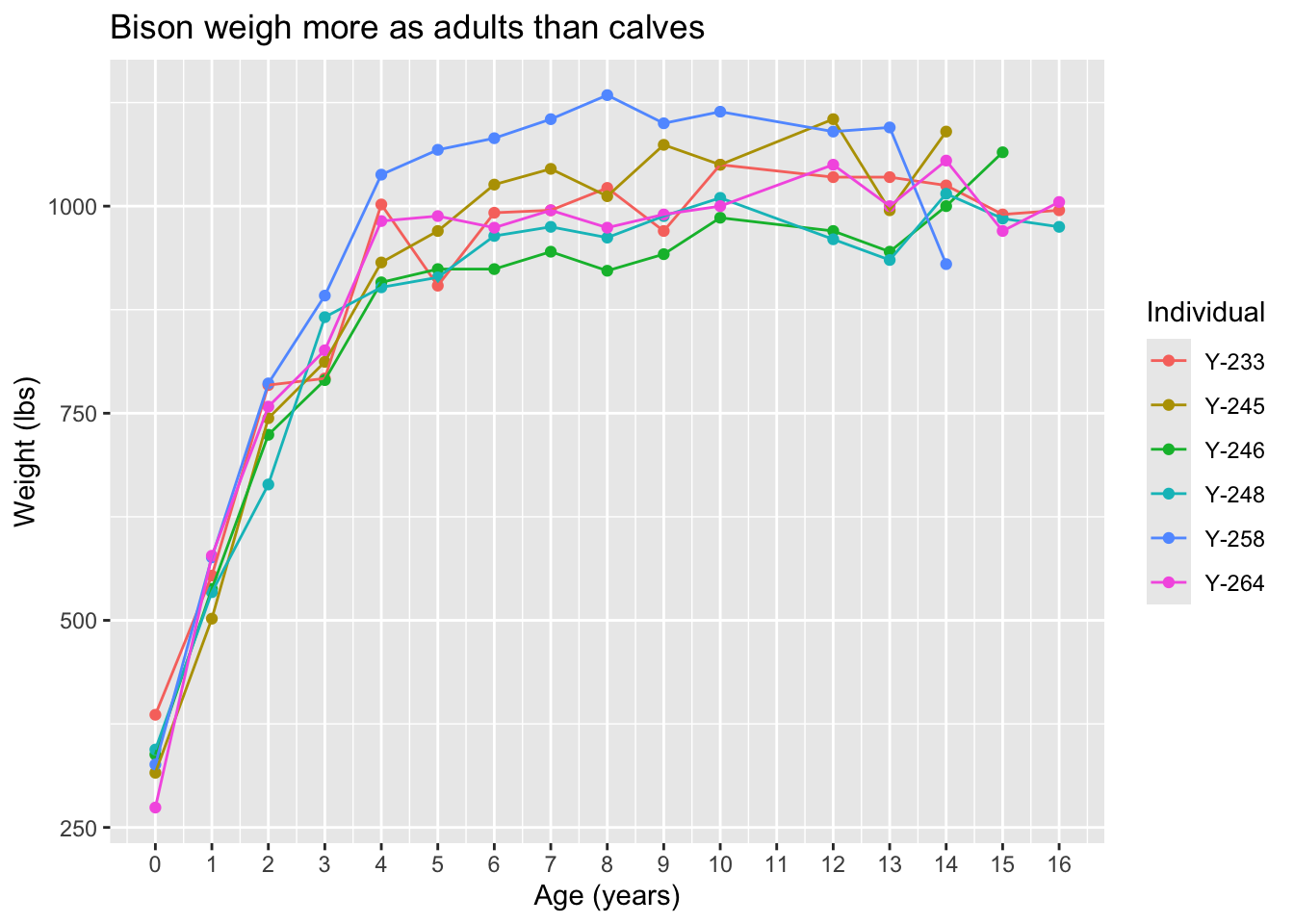

b. North Temperate Lakes ice cover

# creating a plot ----
ntl_ice_plot <- ggplot(data = ntl_icecover, # data
                       aes(x = year, # x-axis
                           y = ice_duration, # y-axis
                           color = lakeid)) + # color by lake
  
  # geometry: line 
  geom_line(aes(group = lakeid), # making sure line is grouped by lake
            linewidth = 1) + # thicker line
  
  # plot appearance
  labs(x = "Year",
       y = "Ice duration (days)",
       title = "Yearly ice duration has declined through time")

ntl_ice_plot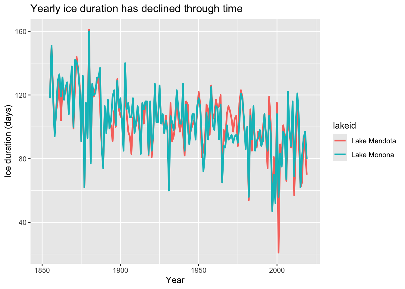

c. Andrews Forest vertebrate species

Figure of length on the x-axis, weight on the y-axis, points representing species observations

# cleaned data frame ----
and_clean <- and_vertebrates %>% # start with and_vertebrates
  filter(species %in% c("Cutthroat trout")) %>% # filter for salamanders and trout
  mutate(unittype = case_when(
    unittype == "C" ~ "Cascade",
    unittype == "P" ~ "Pool",
    unittype == "SC" ~ "Side channel",
    unittype == "IP" ~ "Isolated pools",
    unittype == "R" ~ "Rapid"
  ),
  unittype = fct_relevel(unittype, "Pool", "Cascade", "Rapid", "Side channel", "Isolated pools")) %>% 
  drop_na(unittype)

# creating a plot ----
and_verts_plot <- ggplot(data = and_clean, # use the clean data frame
                         aes(x = unittype, # x-axis
                             y = length_1_mm, # y-axis
                             color = unittype)) + # color the points by species
  
  # drawing points
  geom_boxplot(outliers = FALSE) +
  geom_jitter(width = 0.2,
              height = 0,
              alpha = 0.05,
              shape = 21) +

  
  # plot appearance 
  labs(x = "Habitat type",
       y = "Weight (g)",
       title = "Cutthroat trout in pools are larger than in other habitats") 
 
# displaying the plot ----
and_verts_plot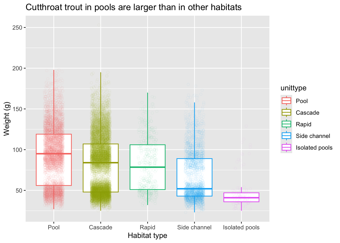

d. Navigate to your section’s slides

These are linked in your workshop template.

3. Advanced figures

a. quick fixes to make your plot better

ntl_ice_quick <- ntl_ice_plot +
  scale_color_manual(values = c("Lake Mendota" = "#6aa84f", 
                                "Lake Monona" = "#45818e")) +
  theme_minimal() +
  theme(text = element_text(size = 16,
                            family = "Times New Roman"),
        axis.text = element_text(color = "#5b5b5b"),
        axis.title = element_text(color = "#5b5b5b"),
        plot.title = element_text(color = "#5b5b5b"),
        legend.position = "bottom",
        legend.title = element_blank())

ntl_ice_quick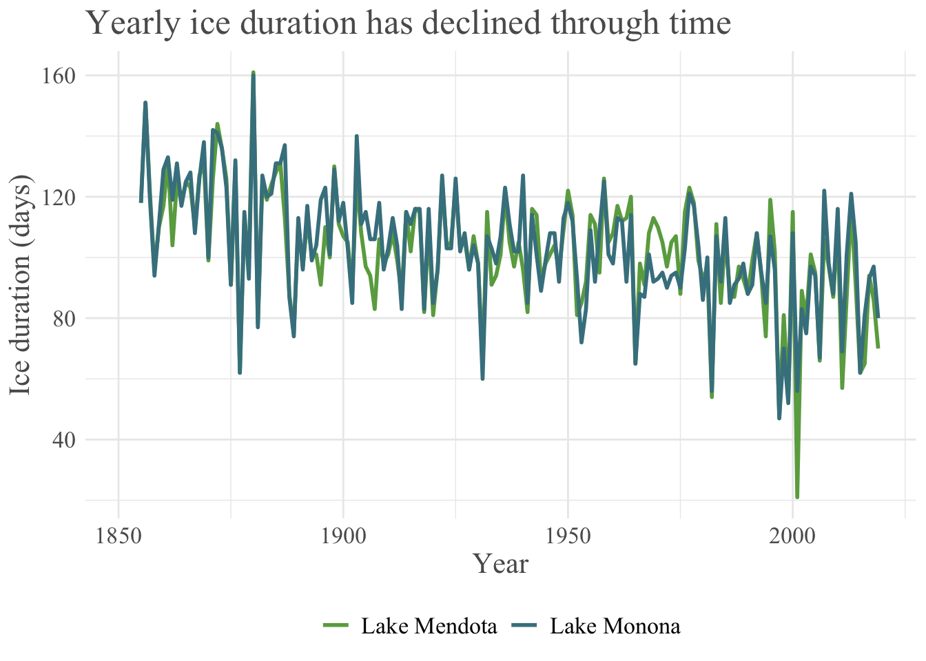

# run this to save your plot!
# ggsave("ntl_ice_quick.png", # what you want your plot file to be called
#        ntl_ice_quick, # plot object name
#        width = 12, # width (change this if necessary)
#        height = 8, # height (change this if necessary)
#        units = cm, # units of width and height
#        dpi = 300) # resolution 

b. use color palettes

and_verts_palette <- and_verts_plot +
  scale_color_manual(values = paletteer_d("peRReo::buenavista")) 

and_verts_palette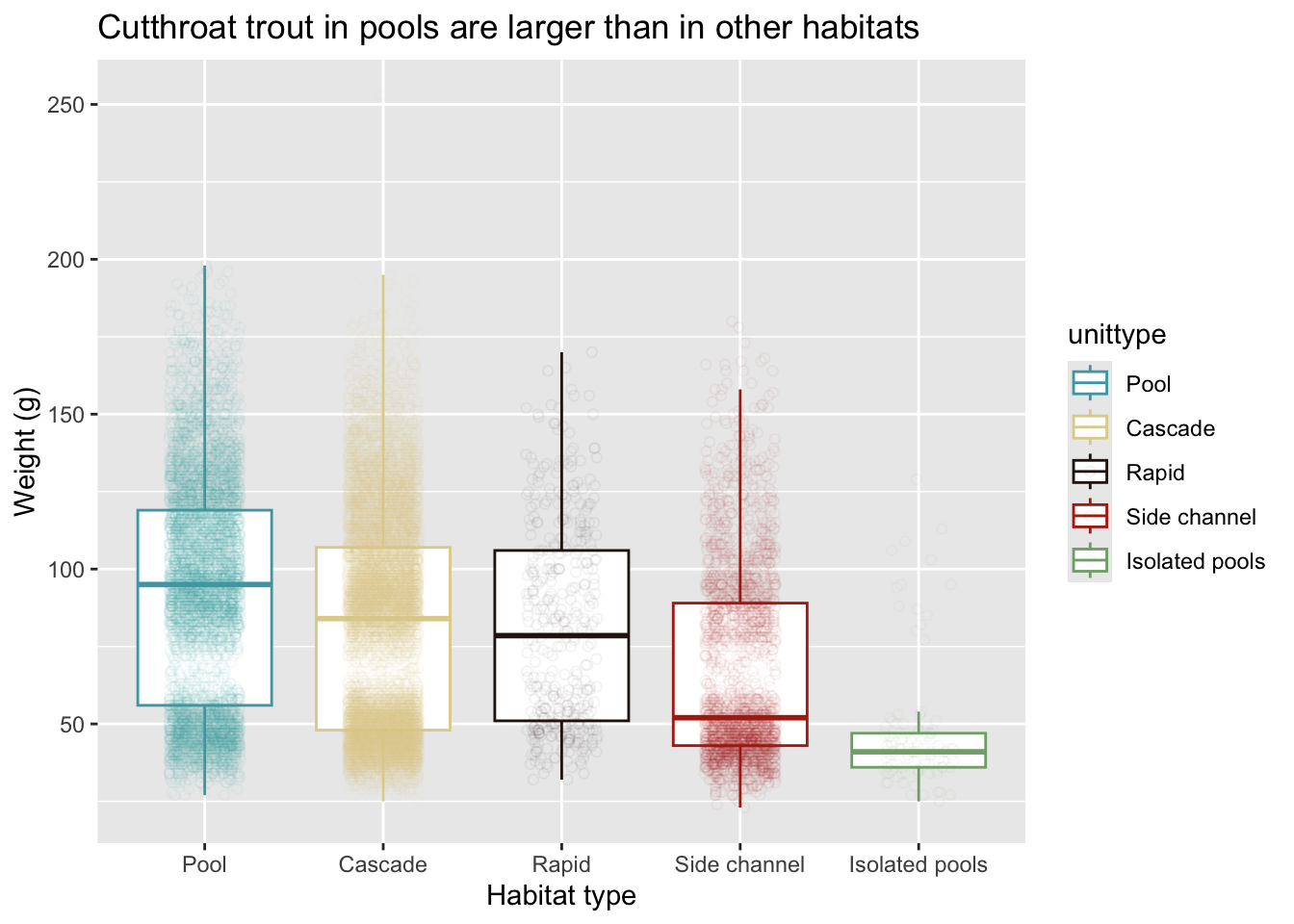

# run this to save your plot!
# ggsave("and_verts_palette.png", # what you want your plot file to be called
#        and_verts_palette, # plot object name
#        width = 10, # width (change this if necessary)
#        height = 8, # height (change this if necessary)
#        units = cm, # units of width and height
#        dpi = 300) # resolution 

c. use theme packages to change plot aesthetics

knz_bison_theme <- knz_bison_plot +
  theme_economist() +
  scale_color_economist()

knz_bison_theme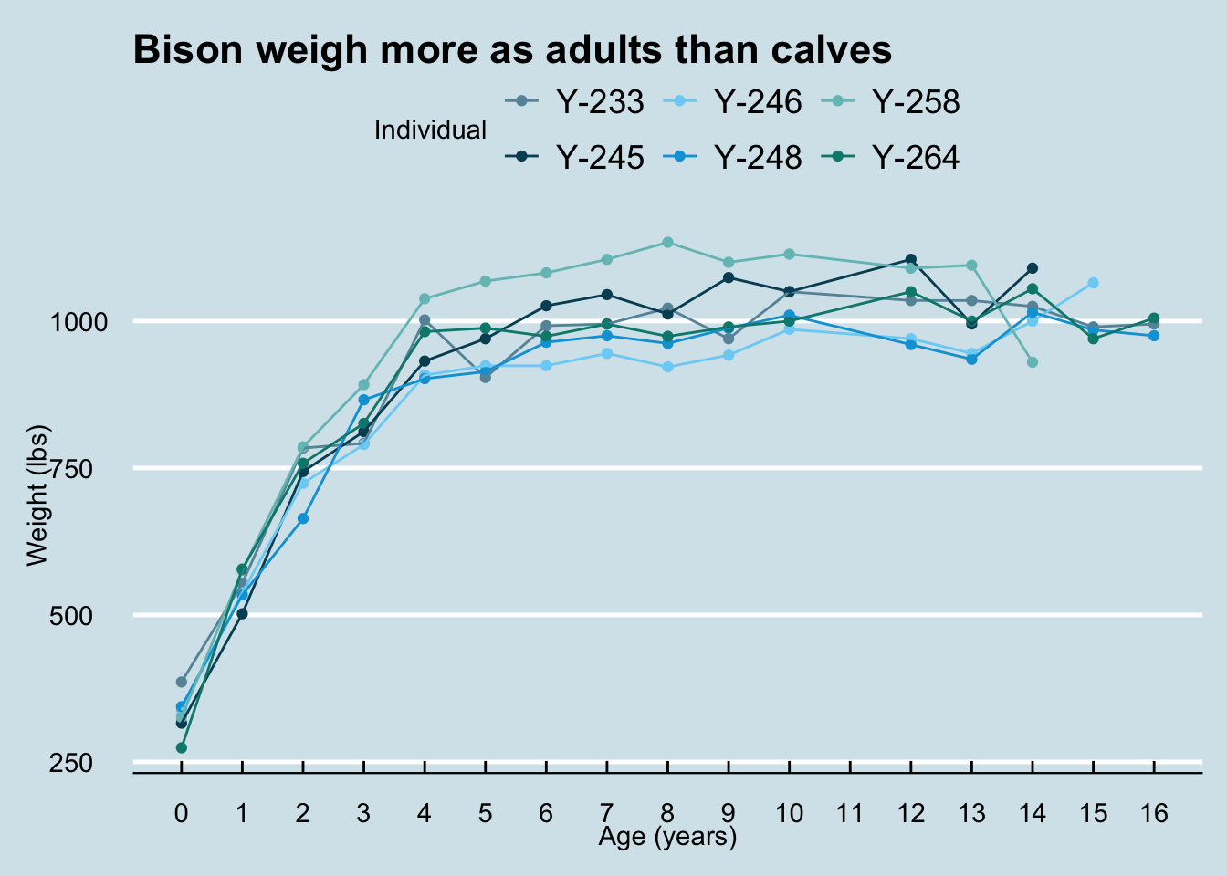

# note that you have to install the "Homemade Apple" font before running this code
# download it here: https://fonts.google.com/share?selection.family=Homemade+Apple
knz_bison_pomological_theme <- knz_bison_plot +
  scale_color_pomological() +
  theme_pomological_fancy()

knz_bison_pomological_theme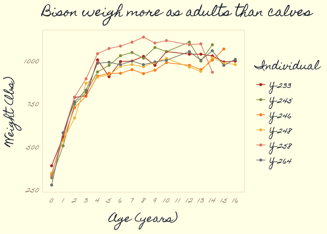

# note that you have to install the "Slayer" font before running this code
# download it here: https://github.com/Ryo-N7/tvthemes/tree/master/inst/fonts/Slayer
# click through to the font, then hit the download button
knz_bison_avatar_theme <- knz_bison_plot +
  scale_color_avatar(palette = "WaterTribe") +
  theme_avatar(title.font = "Slayer",
               text.font = "Slayer",
               title.size = 8,
               subtitle.size = 8)

knz_bison_avatar_theme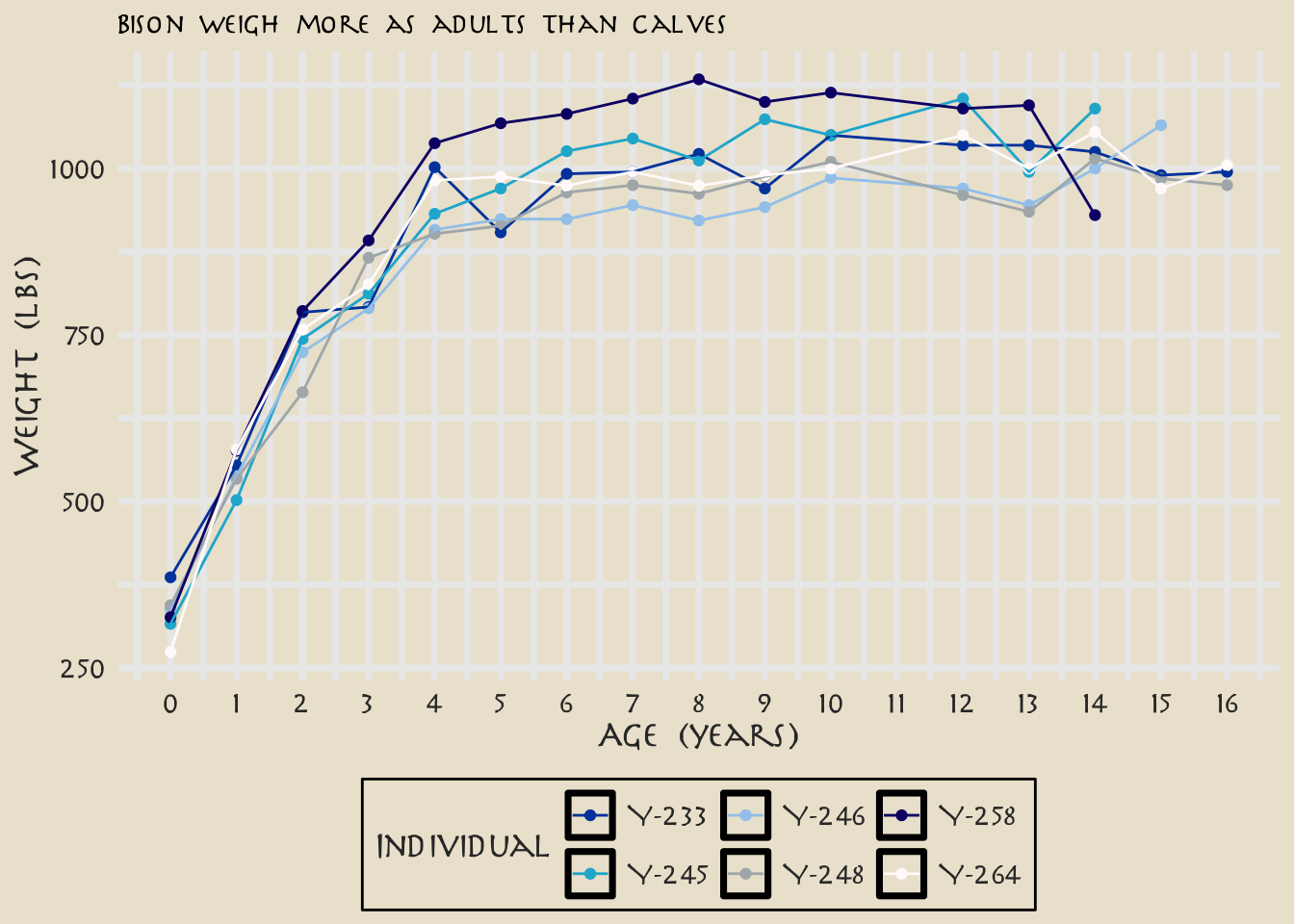

# run this to save your plot!
# ggsave("knz_bison_theme.png", # what you want your plot file to be called
#        knz_bison_theme, # plot object name
#        width = 10, # width (change this if necessary)
#        height = 8, # height (change this if necessary)
#        units = cm, # units of width and height
#        dpi = 300) # resolution 

d. highlight figure components

knz_bison_highlight <- knz_bison_plot +
  gghighlight(animal_code == "Y-233",
              unhighlighted_params = list(alpha = 0.8),
              line_label_type = "ggrepel_label")

knz_bison_highlight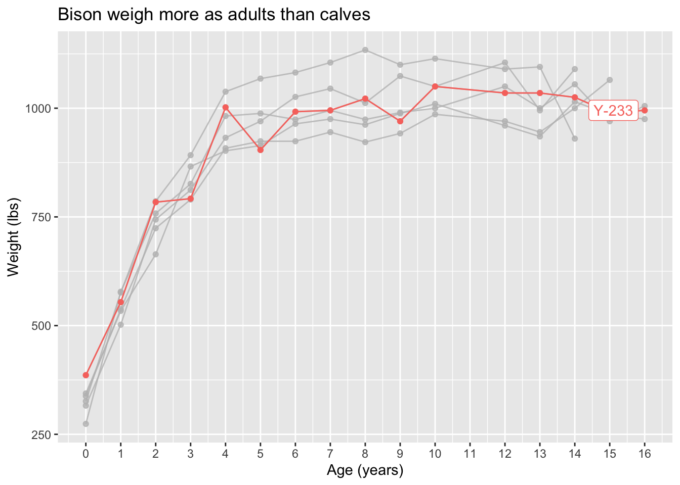 

# run this to save your plot!
# ggsave("knz_bison_highlight.png", # what you want your plot file to be called
#        knz_bison_highlight, # plot object name
#        width = 10, # width (change this if necessary)
#        height = 8, # height (change this if necessary)
#        units = cm, # units of width and height
#        dpi = 300) # resolution 

e. put multiple figures together

plots_together <- ntl_ice_plot / knz_bison_plot

plots_together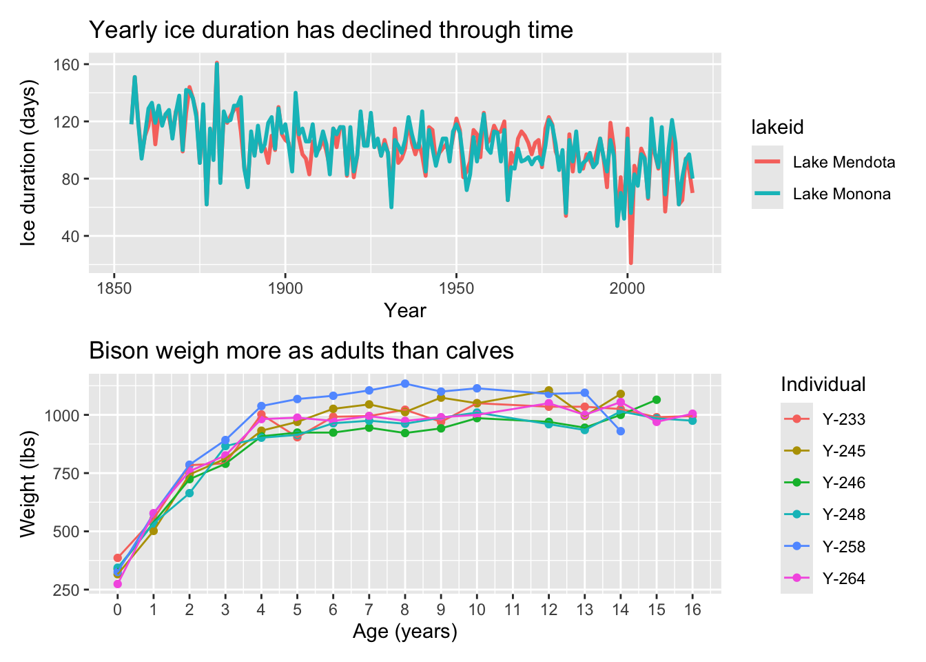

# run this to save your plot!
# ggsave("plots_together.png", # what you want your plot file to be called
#        plots_together, # plot object name
#        width = 12, # width (change this if necessary)
#        height = 10, # height (change this if necessary)
#        units = cm, # units of width and height
#        dpi = 300) # resolution 

f. make figures into gifs

ntl_ice_gif <- ntl_ice_plot +
  transition_reveal(along = year) +
  ease_aes('linear')

ntl_ice_gif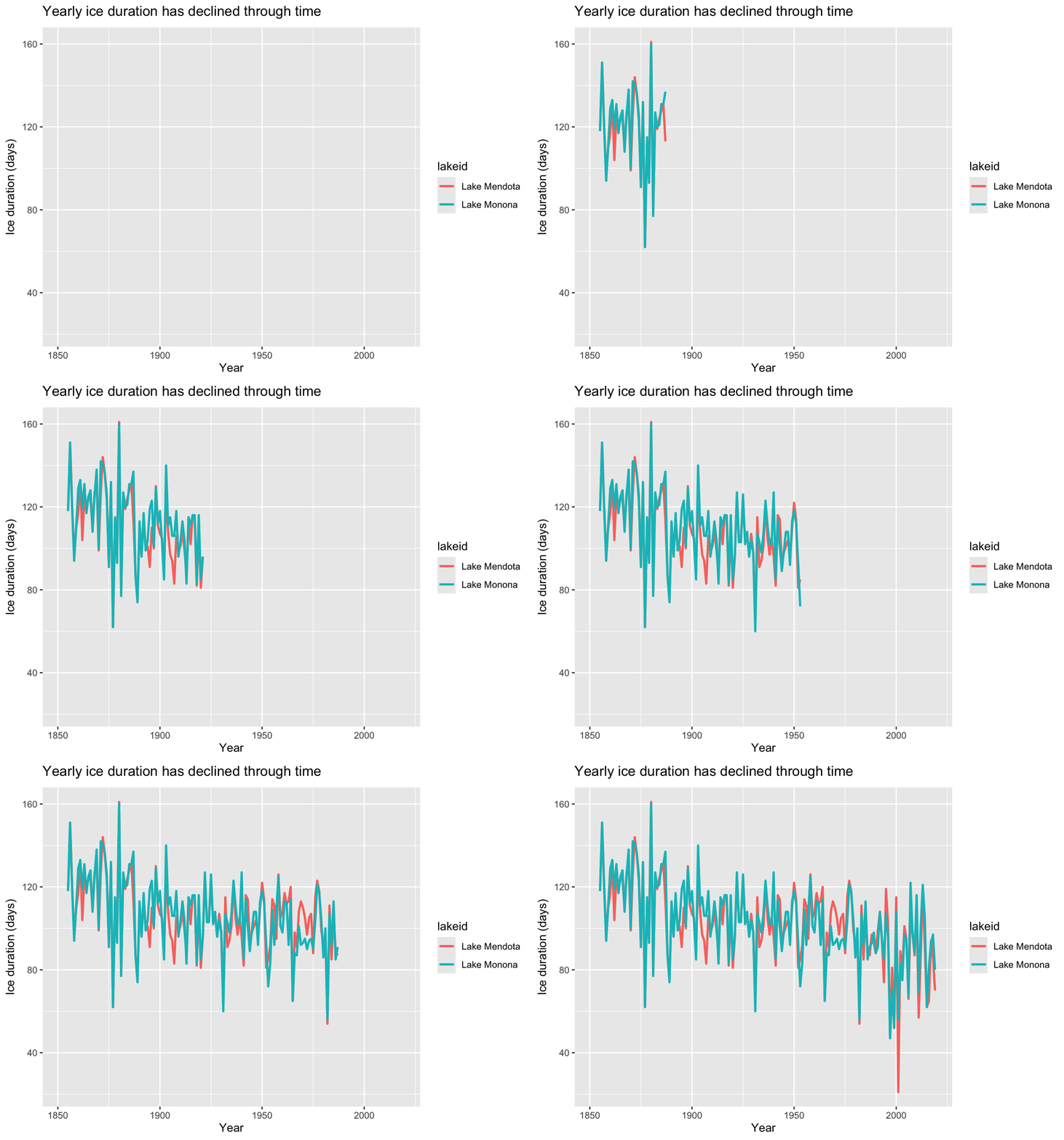

# run this to save your gif!
# anim_save("ntl_ice.gif", 
#           ntl_ice_gif)

g. insert images into plots

Note: if you go with this option, you can use the bison image in this directory with the knz_bison_plot. You can also use a different plot and download another image that makes sense. Up to you!

knz_bison_image <- knz_bison_plot +
  geom_image(
    data = tibble(age = 10, animal_weight = 500),
    aes(image = "bison-on-konza.jpg"),
    size = 0.5
  )

knz_bison_image

# run this to save your plot!
# ggsave("knz_bison_image.png", # what you want your plot file to be called
#        knz_bison_image, # plot object name
#        width = 10, # width (change this if necessary)
#        height = 8, # height (change this if necessary)
#        units = cm, # units of width and height
#        dpi = 300) # resolution 

knz_bison_image <- knz_bison_plot +
  geom_image(
    data = tibble(age = 10, animal_weight = 500),
    aes(image = here::here("workshop", "images", "bison-on-konza.jpg")),
    size = 0.5
  )

knz_bison_image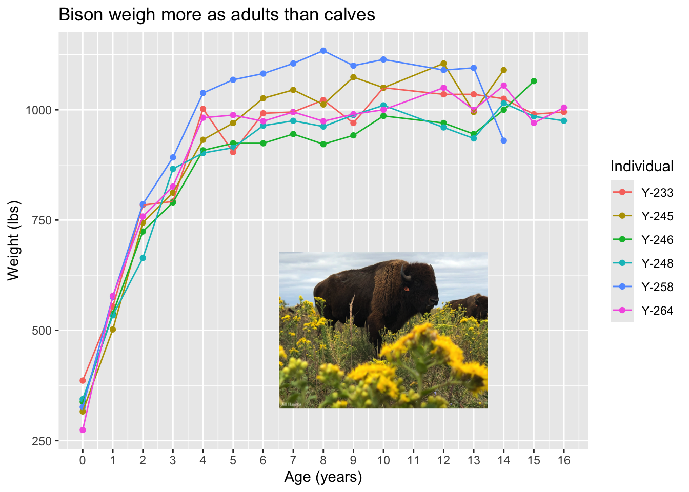

# run this to save your plot!
# ggsave("knz_bison_image.png", # what you want your plot file to be called
#        knz_bison_image, # plot object name
#        width = 10, # width (change this if necessary)
#        height = 8, # height (change this if necessary)
#        units = cm, # units of width and height
#        dpi = 300) # resolution 

h. make figures interactive

ntl_ice_inter <- ggplotly(ntl_ice_plot)

ntl_ice_inter

# run this to save your object!
# htmltools::save_html(ntl_ice_inter,
#                      "ntl_ice_inter.html")