Code

# cleaning
library(tidyverse)
library(readxl)
library(here)
library(janitor)

# visualization
theme_set(theme_classic() +
            theme(panel.grid = element_blank(),
                  axis.text = element_text(size = 18),
                  axis.title = element_text(size = 18),
                  text = element_text(family = "Lato")))
library(patchwork)
library(ggeffects)
library(flextable)
library(GGally)

# data
library(palmerpenguins)

# analysis
library(car)
library(performance)
library(broom)
library(DHARMa)
library(MuMIn)
library(lmtest)
library(equatiomatic)

Code

drought_exp <- read_xlsx(path = here("data", 
                                     "Valliere_etal_EcoApps_Data.xlsx"),
                         sheet = "First Harvest")

# cleaning
drought_exp_clean <- drought_exp %>% 
  clean_names() %>% # nicer column names
  mutate(species_name = case_when( # adding column with species scientific names
    species == "ENCCAL" ~ "Encelia californica", # bush sunflower
    species == "ESCCAL" ~ "Eschscholzia californica", # California poppy
    species == "PENCEN" ~ "Penstemon centranthifolius", # Scarlet bugler
    species == "GRICAM" ~ "Grindelia camporum", # great valley gumweed
    species == "SALLEU" ~ "Salvia leucophylla", # Purple sage
    species == "STIPUL" ~ "Nasella pulchra", # Purple needlegrass
    species == "LOTSCO" ~ "Acmispon glaber" # deerweed
  )) %>% 
  relocate(species_name, .after = species) %>% # moving species_name column after species
  mutate(water_treatment = case_when( # adding column with full treatment names
    water == "WW" ~ "Well watered",
    water == "DS" ~ "Drought stressed"
  )) %>% 
  relocate(water_treatment, .after = water) # moving water_treatment column after water

math

variance inflation factor

The VIF for the \(j^{th}\) predictor is:

\[ VIF_j = \frac{1}{1-R ^2_j} \]

where \(R^2_J\) is the \(R^2\) value obtained by a model with the \(j^{th}\) predictor as a response and the rest of the predictors as predictors.

Code

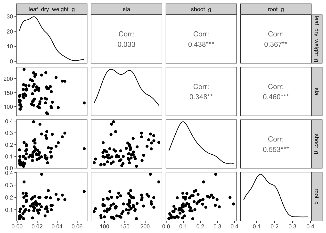
ggpairs(drought_exp_clean, # data frame
        columns = c("leaf_dry_weight_g", # columns to visualize
                    "sla", 
                    "shoot_g", 
                    "root_g"), 
        upper = list(method = "pearson")) + # calculating Pearson correlation coefficient
  theme_bw() + # cleaner theme
  theme(panel.grid = element_blank()) # getting rid of gridlines

VIF

Code

plant_model_all <- lm(total_g ~ leaf_dry_weight_g + sla + root_g + shoot_g,
                      data = drought_exp_clean)

vif(plant_model_all)

leaf_dry_weight_g               sla            root_g           shoot_g 
         1.333854          1.351758          1.724823          1.645045

Code

plant_model_simple <- lm(total_g ~ leaf_dry_weight_g + sla + r_s,
                         data = drought_exp_clean)

vif(plant_model_simple)

leaf_dry_weight_g               sla               r_s 
         1.049871          1.001752          1.049834

Code

model1 <- lm(total_g ~ sla + water_treatment + species,
             data = drought_exp_clean)

vif(model1)

                    GVIF Df GVIF^(1/(2*Df))
sla             4.900028  1        2.213601
water_treatment 1.367759  1        1.169512
species         4.532269  6        1.134209

interaction terms

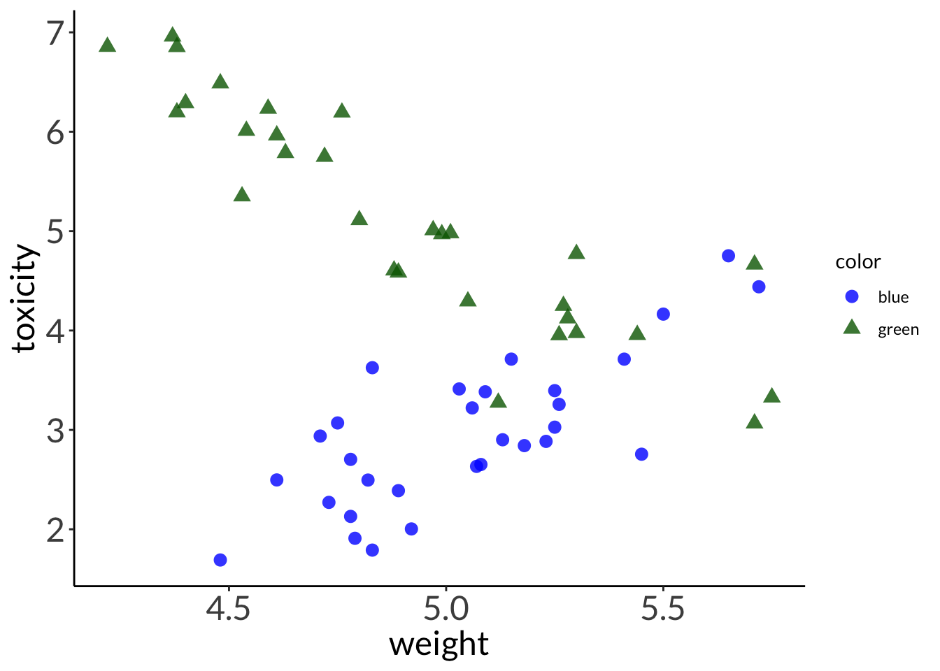
using a modified version of the frog toxicity model

no interaction

Code

frog_num <- 30
set.seed(666)
frogs <- tibble(
  weight = c(
    round(rnorm(n = frog_num, mean = 5, sd = 0.35), 2),
    round(rnorm(n = frog_num, mean = 5, sd = 0.35), 2)
  ),
  color = c(
    rep("green", frog_num),
    rep("blue", frog_num)
  )
) %>% 
  mutate(toxicity = case_when(
    color == "green" ~ round(rnorm(n = frog_num, mean = 2, sd = 0.1), 2)*weight - 5,
    color == "blue" ~ round(rnorm(n = frog_num, mean = 2, sd = 0.1), 2)*weight - 3
  ))

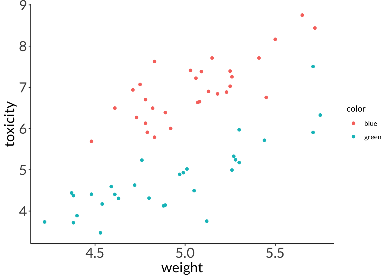
ggplot(data = frogs,
       aes(x = weight,
           y = toxicity,
           color = color)) +
  geom_point()

Code

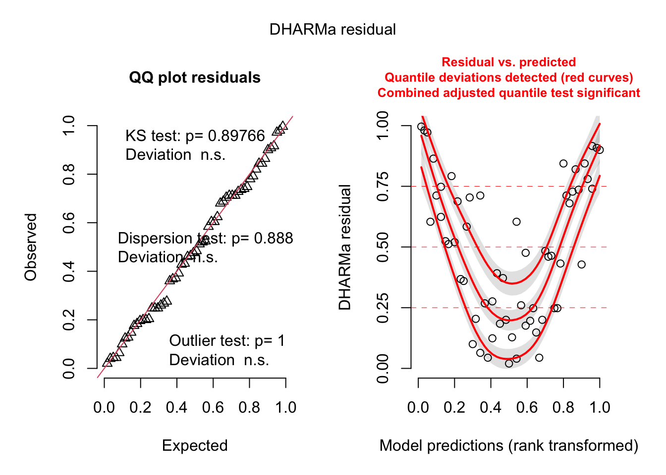
frog_mod <- lm(toxicity ~ weight + color,
               data = frogs)

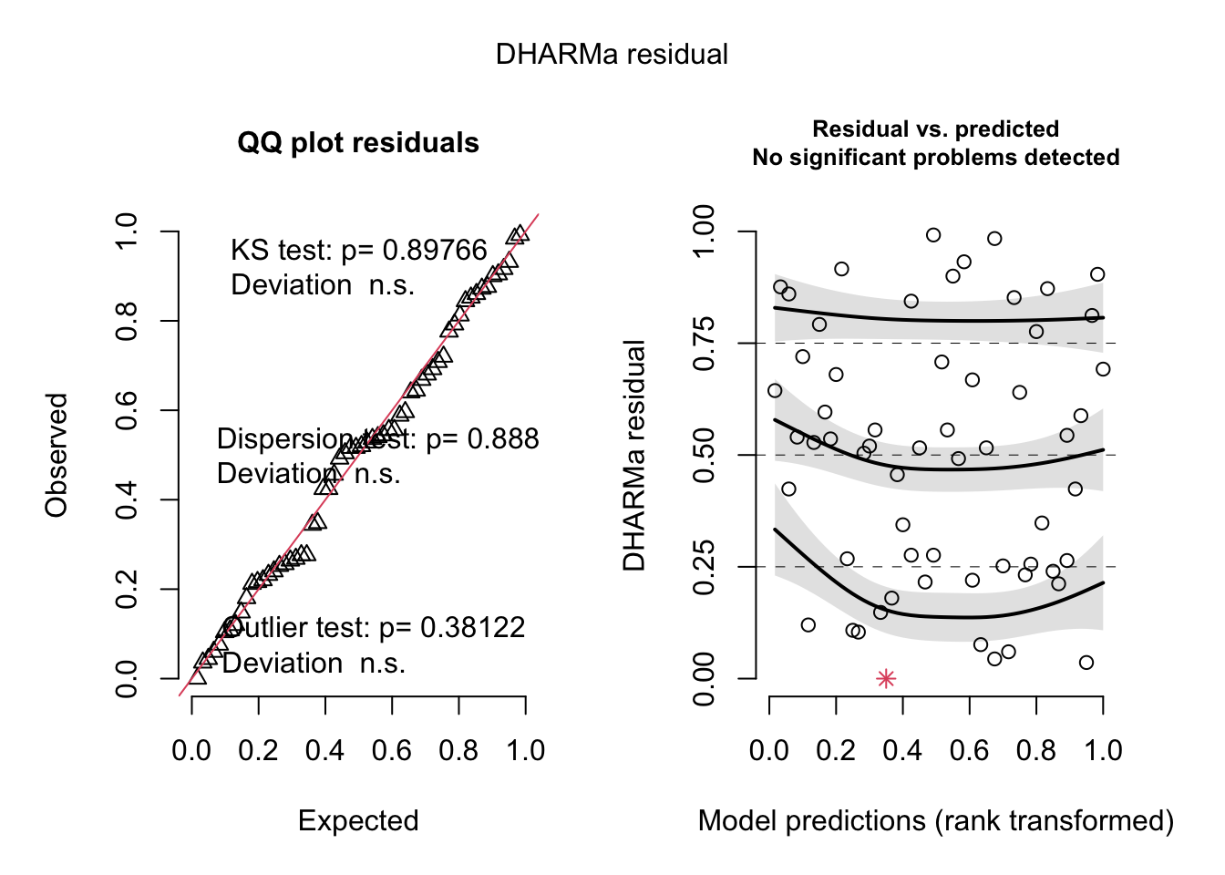
simulateResiduals(frog_mod) %>% plot()

Code

summary(frog_mod)


Call:
lm(formula = toxicity ~ weight + color, data = frogs)

Residuals:
     Min       1Q   Median       3Q      Max 
-1.38164 -0.30495  0.01705  0.32444  1.34105 

Coefficients:
            Estimate Std. Error t value Pr(>|t|)    
(Intercept)  -1.8311     0.8863  -2.066   0.0434 *  
weight        1.7407     0.1747   9.966 4.26e-14 ***
colorgreen   -1.9444     0.1311 -14.834  < 2e-16 ***
---
Signif. codes:  0 '***' 0.001 '**' 0.01 '*' 0.05 '.' 0.1 ' ' 1

Residual standard error: 0.4992 on 57 degrees of freedom
Multiple R-squared:  0.8713,    Adjusted R-squared:  0.8668 
F-statistic: 192.9 on 2 and 57 DF,  p-value: < 2.2e-16

Code

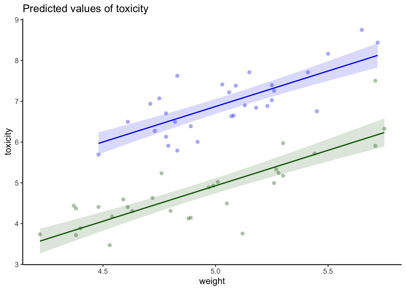
ggpredict(frog_mod,
          terms = c("weight [all]",
                    "color")) %>% 
  plot(show_data = TRUE, 
       limit_range = TRUE) +
  scale_color_manual(values = c("green" = "darkgreen", 
                                "blue" = "blue")) +
  scale_fill_manual(values = c("green" = "darkgreen", 
                                "blue" = "blue")) +
  theme_classic() +
  theme(legend.position = "none")

with interaction

Code

set.seed(666)
frogs <- tibble(
  weight = c(
    round(rnorm(n = frog_num, mean = 5, sd = 0.35), 2),
    round(rnorm(n = frog_num, mean = 5, sd = 0.35), 2)
  ),
  color = c(
    rep("green", frog_num),
    rep("blue", frog_num)
  )
) %>% 
  mutate(toxicity = case_when(
    color == "green" ~ round(rnorm(n = frog_num, mean = -2, sd = 0.1), 2)*weight + 15,
    color == "blue" ~ round(rnorm(n = frog_num, mean = 2, sd = 0.1), 2)*weight - 7
  ))

ggplot(data = frogs,
       aes(x = weight,
           y = toxicity,
           color = color,
           shape = color)) +
  geom_point(size = 3,
             alpha = 0.8) +
  # scale_x_continuous(limits = c(0, 7)) +
  scale_color_manual(values = c("green" = "darkgreen", 
                                "blue" = "blue"))

Code

frog_mod1 <- lm(toxicity ~ weight + color, # no interaction
               data = frogs)

frog_mod2 <- lm(toxicity ~ weight * color, # interaction
               data = frogs)

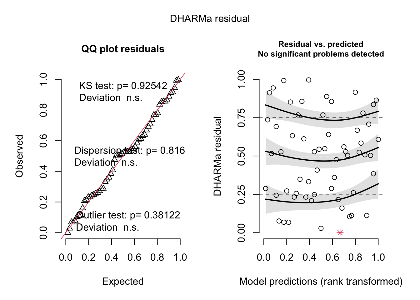
simulateResiduals(frog_mod1) %>% plot() # no interaction

Code

simulateResiduals(frog_mod2) %>% plot() # interaction

Code

summary(frog_mod1) # no interaction


Call:
lm(formula = toxicity ~ weight + color, data = frogs)

Residuals:
     Min       1Q   Median       3Q      Max 
-1.78880 -0.67346 -0.02757  0.54386  2.35344 

Coefficients:
            Estimate Std. Error t value Pr(>|t|)    
(Intercept)   7.6209     1.5994   4.765 1.34e-05 ***
weight       -0.9243     0.3152  -2.933  0.00483 ** 
colorgreen    2.0470     0.2365   8.655 5.69e-12 ***
---
Signif. codes:  0 '***' 0.001 '**' 0.01 '*' 0.05 '.' 0.1 ' ' 1

Residual standard error: 0.9008 on 57 degrees of freedom
Multiple R-squared:  0.6272,    Adjusted R-squared:  0.6141 
F-statistic: 47.94 on 2 and 57 DF,  p-value: 6.135e-13

Code

summary(frog_mod2) # interaction


Call:
lm(formula = toxicity ~ weight * color, data = frogs)

Residuals:
     Min       1Q   Median       3Q      Max 
-1.36733 -0.31151  0.01057  0.35051  1.39586 

Coefficients:
                  Estimate Std. Error t value Pr(>|t|)    
(Intercept)        -6.5225     1.5382  -4.240 8.44e-05 ***
weight              1.8777     0.3042   6.172 7.96e-08 ***
colorgreen         23.0841     1.8689  12.352  < 2e-16 ***
weight:colorgreen  -4.2056     0.3727 -11.285 4.78e-16 ***
---
Signif. codes:  0 '***' 0.001 '**' 0.01 '*' 0.05 '.' 0.1 ' ' 1

Residual standard error: 0.5023 on 56 degrees of freedom
Multiple R-squared:  0.8861,    Adjusted R-squared:   0.88 
F-statistic: 145.3 on 3 and 56 DF,  p-value: < 2.2e-16

Code

model.sel(frog_mod1, # no interaction
          frog_mod2) # interaction

Model selection table 
           (Int) clr       wgh clr:wgh df  logLik  AICc delta
frog_mod2 -6.523   + 1.000e+00       +  5 -41.749  94.6  0.00
frog_mod1  7.621   + 1.162e-15          4 -77.329 163.4 68.78
Models ranked by AICc(x)

Code

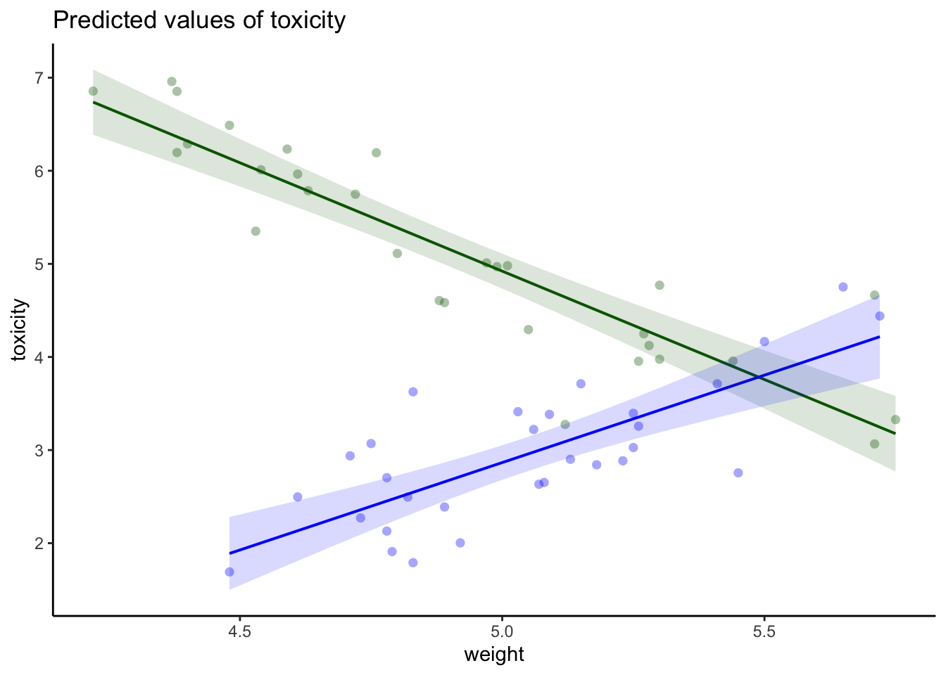
ggpredict(frog_mod2,
          terms = c("weight [all]",
                    "color")) %>% 
  plot(show_data = TRUE, 
       limit_range = TRUE) +
  scale_color_manual(values = c("green" = "darkgreen", 
                                "blue" = "blue")) +
  scale_fill_manual(values = c("green" = "darkgreen", 
                                "blue" = "blue")) +
  theme_classic() +
  theme(legend.position = "none")

calculating slopes (very hacky):

Code

predictions <- ggpredict(frog_mod2,
          terms = c("weight [all]",
                    "color")) %>% 
  group_by(group) %>% 
  filter(predicted %in% c(max(predicted), min(predicted))) %>% 
  arrange(group)

predictions

# A tibble: 4 × 6
# Groups:   group [2]
      x predicted std.error conf.low conf.high group
  <dbl>     <dbl>     <dbl>    <dbl>     <dbl> <fct>
1  4.22      6.74     0.175    6.39       7.09 green
2  5.75      3.18     0.203    2.77       3.58 green
3  4.22      1.40     0.268    0.864      1.94 blue 
4  5.75      4.27     0.232    3.81       4.74 blue

Code

# solve for slopes
green_slope <- (pluck(predictions, 2, 2) - pluck(predictions, 2, 1))/(pluck(predictions, 1, 2) - pluck(predictions, 1, 1))
green_slope

[1] -2.327946

Code

blue_slope <- (pluck(predictions, 2, 4) - pluck(predictions, 2, 3))/(pluck(predictions, 1, 4) - pluck(predictions, 1, 3))
blue_slope

[1] 1.877666

Code

# solve for intercepts
green_intercept <- pluck(predictions, 2, 2) - (green_slope*pluck(predictions, 1, 2))
green_intercept

[1] 16.56161

Code

blue_intercept <- pluck(predictions, 2, 4) - (blue_slope*pluck(predictions, 1, 4))
blue_intercept

[1] -6.522534

Code

ggpredict(frog_mod2,
          terms = c("weight [5]",
                    "color"))

# Predicted values of toxicity

color: green

weight | Predicted |     95% CI
-------------------------------
     5 |      4.92 | 4.73, 5.11

color: blue

weight | Predicted |     95% CI
-------------------------------
     5 |      2.87 | 2.68, 3.05

Code

green_slope*5 + green_intercept

[1] 4.921879

Code

blue_slope*5 + blue_intercept

[1] 2.865798

simpson’s paradox

Code

bill_model <- lm(bill_length_mm ~ bill_depth_mm, data = penguins)

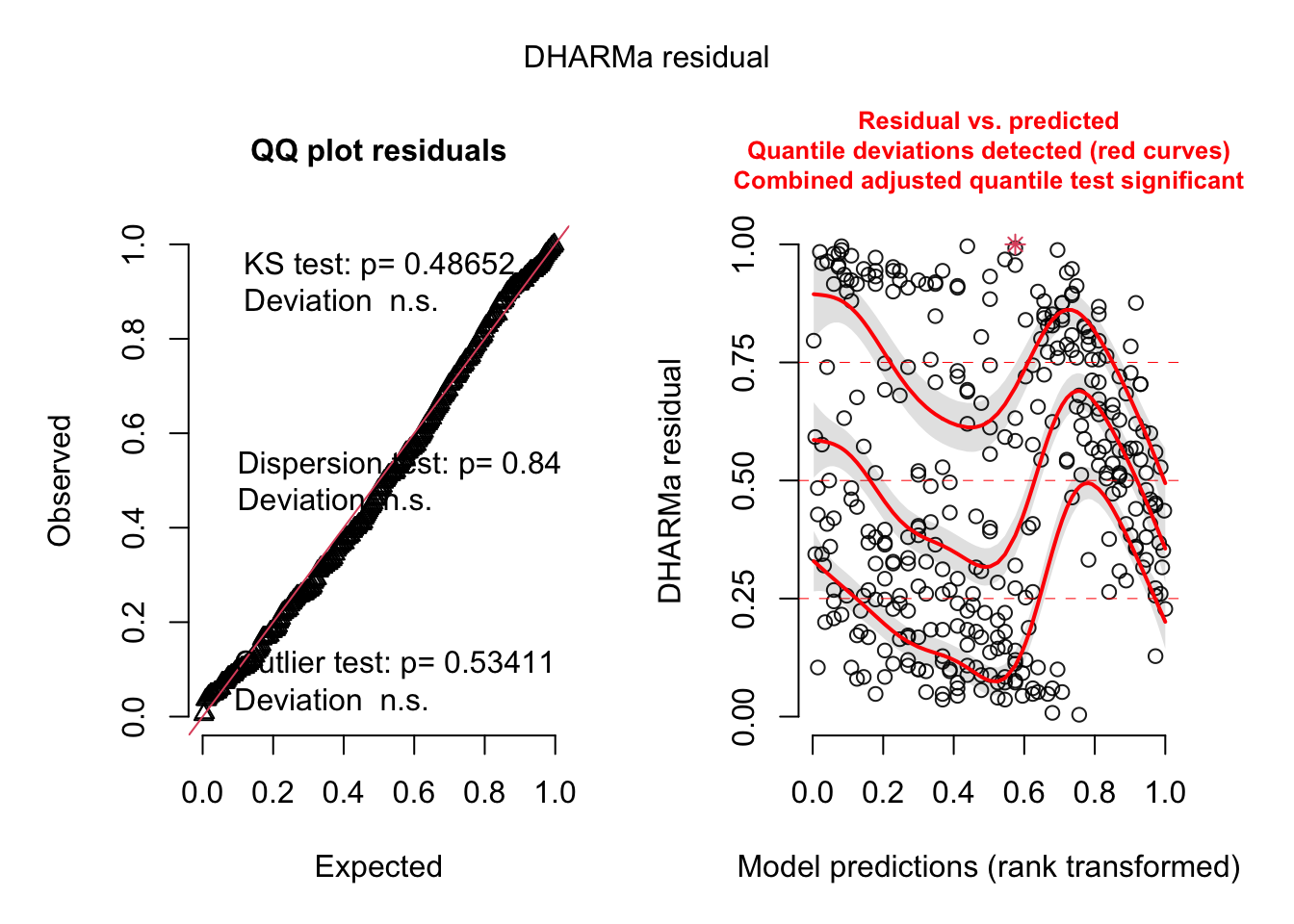
simulateResiduals(bill_model) %>% plot()

Code

summary(bill_model)


Call:
lm(formula = bill_length_mm ~ bill_depth_mm, data = penguins)

Residuals:
     Min       1Q   Median       3Q      Max 
-12.8949  -3.9042  -0.3772   3.6800  15.5798 

Coefficients:
              Estimate Std. Error t value Pr(>|t|)    
(Intercept)    55.0674     2.5160  21.887  < 2e-16 ***
bill_depth_mm  -0.6498     0.1457  -4.459 1.12e-05 ***
---
Signif. codes:  0 '***' 0.001 '**' 0.01 '*' 0.05 '.' 0.1 ' ' 1

Residual standard error: 5.314 on 340 degrees of freedom
  (2 observations deleted due to missingness)
Multiple R-squared:  0.05525,   Adjusted R-squared:  0.05247 
F-statistic: 19.88 on 1 and 340 DF,  p-value: 1.12e-05

Code

confint(bill_model)

                   2.5 %     97.5 %
(Intercept)   50.1185795 60.0161600
bill_depth_mm -0.9364867 -0.3631844

Code

bill_model_preds <- ggpredict(bill_model, terms = "bill_depth_mm")

model_plot <- ggplot(penguins, aes(x = bill_depth_mm, y = bill_length_mm)) +
  geom_point() +
  geom_line(data = bill_model_preds, aes(x = x, y = predicted), color = "blue", linewidth = 2) +
  geom_ribbon(data = bill_model_preds, aes(x = x, y = predicted, ymin = conf.low, ymax = conf.high), alpha = 0.2) +
  theme_classic() +
  labs(x = "Bill depth (mm)", y = "Bill length (mm)")

\[ length = -0.65*depth + 55.07 \]

Code

bill_model2 <- lm(bill_length_mm ~ bill_depth_mm*species, data = penguins)
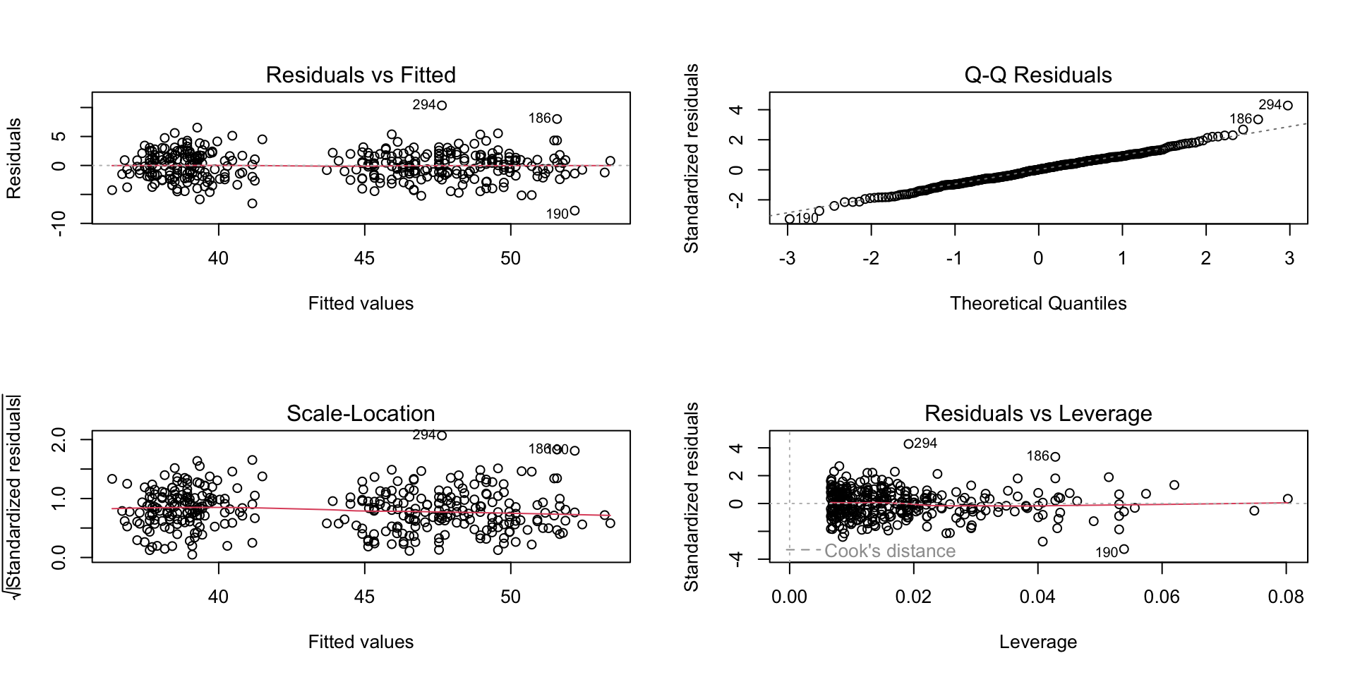
par(mfrow = c(2, 2))
plot(bill_model2)

Code

summary(bill_model2)


Call:
lm(formula = bill_length_mm ~ bill_depth_mm * species, data = penguins)

Residuals:
    Min      1Q  Median      3Q     Max 
-7.7888 -1.5415  0.0575  1.5873 10.3590 

Coefficients:
                               Estimate Std. Error t value Pr(>|t|)    
(Intercept)                     23.0681     3.0165   7.647 2.18e-13 ***
bill_depth_mm                    0.8570     0.1641   5.224 3.08e-07 ***
speciesChinstrap                -9.6402     5.7154  -1.687 0.092590 .  
speciesGentoo                   -5.8386     4.5353  -1.287 0.198850    
bill_depth_mm:speciesChinstrap   1.0651     0.3100   3.435 0.000666 ***
bill_depth_mm:speciesGentoo      1.1637     0.2789   4.172 3.84e-05 ***
---
Signif. codes:  0 '***' 0.001 '**' 0.01 '*' 0.05 '.' 0.1 ' ' 1

Residual standard error: 2.445 on 336 degrees of freedom
  (2 observations deleted due to missingness)
Multiple R-squared:  0.8024,    Adjusted R-squared:  0.7995 
F-statistic: 272.9 on 5 and 336 DF,  p-value: < 2.2e-16

Code

lrtest(bill_model2)

Likelihood ratio test

Model 1: bill_length_mm ~ bill_depth_mm * species
Model 2: bill_length_mm ~ 1
  #Df   LogLik Df  Chisq Pr(>Chisq)    
1   7  -787.97                         
2   2 -1065.28 -5 554.62  < 2.2e-16 ***
---
Signif. codes:  0 '***' 0.001 '**' 0.01 '*' 0.05 '.' 0.1 ' ' 1

Code

anova(bill_model2)

Analysis of Variance Table

Response: bill_length_mm
                       Df Sum Sq Mean Sq F value    Pr(>F)    
bill_depth_mm           1  561.6   561.6  93.965 < 2.2e-16 ***
species                 2 7460.3  3730.2 624.151 < 2.2e-16 ***
bill_depth_mm:species   2  134.3    67.1  11.232 1.898e-05 ***
Residuals             336 2008.1     6.0                      
---
Signif. codes:  0 '***' 0.001 '**' 0.01 '*' 0.05 '.' 0.1 ' ' 1

Code

waldtest(bill_model2)

Wald test

Model 1: bill_length_mm ~ bill_depth_mm * species
Model 2: bill_length_mm ~ 1
  Res.Df Df      F    Pr(>F)    
1    336                        
2    341 -5 272.95 < 2.2e-16 ***
---
Signif. codes:  0 '***' 0.001 '**' 0.01 '*' 0.05 '.' 0.1 ' ' 1

Code

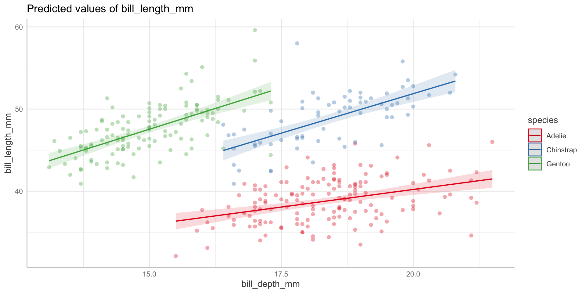
ggpredict(bill_model2, 
          terms = c("bill_depth_mm [all]", 
                    "species")) %>% 
  plot(show_data = TRUE, 
       limit_range = TRUE)

Code

penguins %>% 
  group_by(species) %>% 
  summarize(min = min(bill_depth_mm, na.rm = TRUE),
            max = max(bill_depth_mm, na.rm = TRUE))

# A tibble: 3 × 3
  species     min   max
  <fct>     <dbl> <dbl>
1 Adelie     15.5  21.5
2 Chinstrap  16.4  20.8
3 Gentoo     13.1  17.3

Code

bill_model2_preds <- ggpredict(bill_model2, 
                               terms = c("bill_depth_mm [13.1:21.5 by = 0.1]", 
                                         "species")) %>% 
  as_tibble() %>% 
  rename(species = group) %>% 
  mutate(keep = case_when(
    species == "Adelie" & between(x, 15.5, 21.5) ~ "keep",
    species == "Chinstrap" & between(x, 16.4, 20.8) ~ "keep",
    species == "Gentoo" & between(x, 13.1, 17.3) ~ "keep"
  )) %>% 
  drop_na(keep) %>% 
  select(-keep)

model2_plot <- ggplot(penguins, 
                      aes(x = bill_depth_mm, 
                          y = bill_length_mm)) +
  geom_point(aes(color = species)) +
  geom_line(data = bill_model2_preds, 
            aes(x = x, 
                y = predicted, 
                color = species), 
            linewidth = 2) +
  geom_ribbon(data = bill_model2_preds, 
              aes(x = x, 
                  y = predicted, 
                  ymin = conf.low, 
                  ymax = conf.high, 
                  fill = species), 
              alpha = 0.2) +
  scale_color_manual(values = c("cornflowerblue", "darkgreen", "darkorange")) +
  scale_fill_manual(values = c("cornflowerblue", "darkgreen", "darkorange")) +
  theme_classic() +
  labs(x = "Bill depth (mm)", 
       y = "Bill length (mm)",
       color = "Species", 
       fill = "Species") 

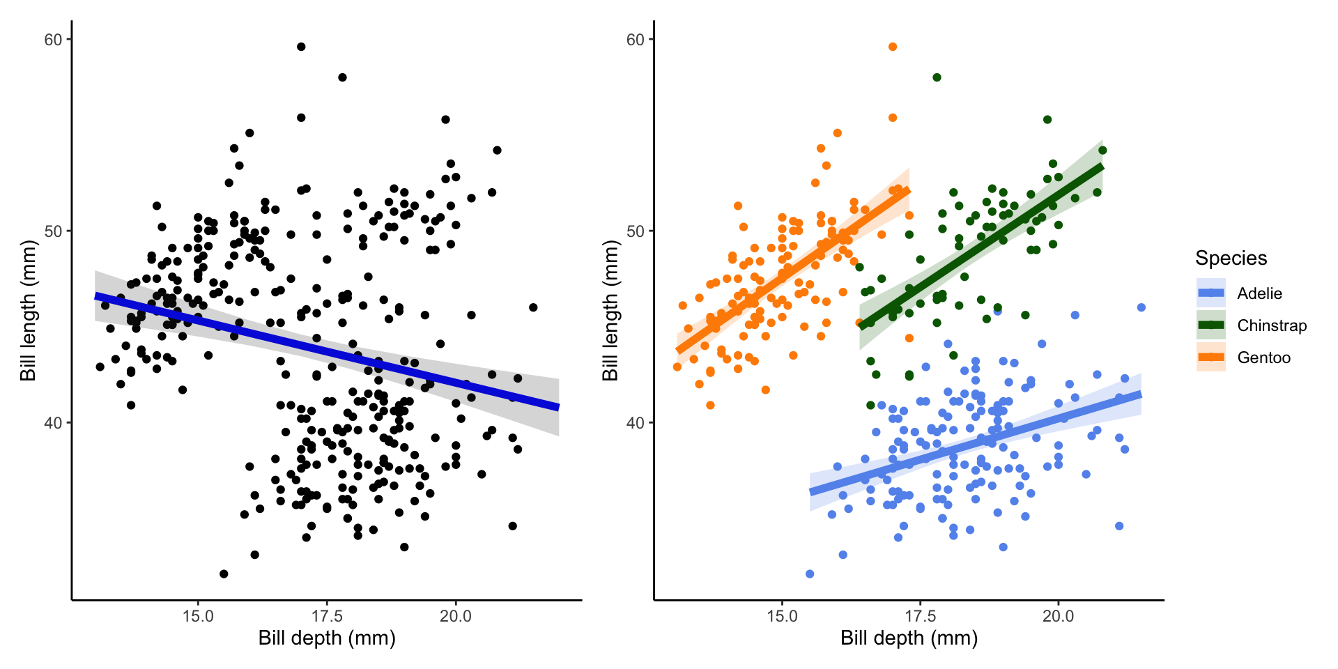
model_plot + model2_plot

Code

extract_eq(bill_model)

\[ \operatorname{bill\_length\_mm} = \alpha + \beta_{1}(\operatorname{bill\_depth\_mm}) + \epsilon \]

\[ \operatorname{bill\_length\_mm} = \alpha + \beta_{1}(\operatorname{bill\_depth\_mm}) + \beta_{2}(\operatorname{species}_{\operatorname{Chinstrap}}) + \beta_{3}(\operatorname{species}_{\operatorname{Gentoo}}) + \beta_{4}(\operatorname{bill\_depth\_mm} \times \operatorname{species}_{\operatorname{Chinstrap}}) + \beta_{5}(\operatorname{bill\_depth\_mm} \times \operatorname{species}_{\operatorname{Gentoo}}) + \epsilon \]

\[ \operatorname{bill\_length\_mm} = \alpha + \beta_{1}(\operatorname{bill\_depth\_mm}) + \epsilon \]

Citation

BibTeX citation:

@online{bui2024,
  author = {Bui, An},
  title = {Week 9 Figures - {Lecture} 16},
  date = {2024-05-29},
  url = {https://spring-2024.envs-193ds.com/lecture/lecture_week-08.html},
  langid = {en}
}

For attribution, please cite this work as:

Bui, An. 2024. “Week 9 Figures - Lecture 16.” May 29, 2024. https://spring-2024.envs-193ds.com/lecture/lecture_week-08.html.